Specifying models with demes

New in version 1.1, moments can compute the SFS and LD statistics directly from a demes-formatted demographic model. To learn about how to describe a demographic model using demes, head to the demes repository or documentation to learn about specifying multi-population demographic models using demes.

What is demes?

Demographic models specify the historical size changes, migrations, splits and mergers of related populations. Specifying demographic models using moments or practically any other simulation engine can become very complicated and error prone, especially when we want to model more than one population (e.g. [Ragsdale2020]). Even worse, every individual software has its own language and methods for specifying a demographic model, so a user has to reimplement the same model across multiple software, which nobody enjoys. To resolve these issues of reproducibility, replication, and susceptibility to errors, demes provides a human-readable specification of complex demography that is designed to make it easier to implement and share models and to be able to use that demography with multiple simulation engines.

Demes models are written in YAML, and they are then automatically parsed to create an internal representation of the demography that is readable by moments. moments can then iterate through the epochs and demographic events in that model and compute the SFS or LD.

Simulating the SFS and LD using a demes model

Computing expectations for the SFS or LD using a demes model is designed to be as simple as possible. In fact, there is no need for the user to specify any demographic events or integrate the SFS or LD objects. moments does all of that for you.

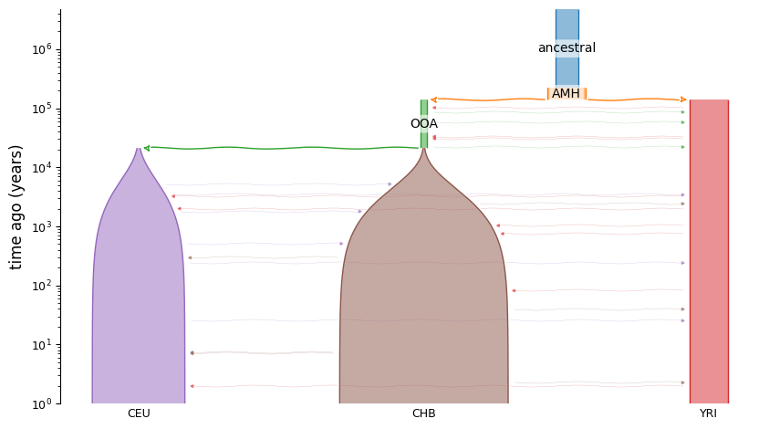
It’s easiest to see the functionality through example. In the tests directory, there is a YAML description of the [Gutenkunst2009] Out-of-African model:

description: The Gutenkunst et al. (2009) three-population model of human history.
doi:
  - https://doi.org/10.1371/journal.pgen.1000695
time_units: years
generation_time: 25
demes:
  - name: ancestral
    description: Equilibrium/root population
    epochs:
    - end_time: 220e3
      start_size: 7300
  - name: AMH
    description: Anatomically modern humans
    ancestors: [ancestral]
    epochs:
    - end_time: 140e3
      start_size: 12300
  - name: OOA
    description: Bottleneck out-of-Africa population
    ancestors: [AMH]
    epochs:
    - end_time: 21.2e3
      start_size: 2100
  - name: YRI
    description: Yoruba in Ibadan, Nigeria
    ancestors: [AMH]
    epochs:
    - start_size: 12300
      end_time: 0
  - name: CEU
    description: Utah Residents (CEPH) with Northern and Western European Ancestry
    ancestors: [OOA]
    epochs:
    - start_size: 1000
      end_size: 29725
      end_time: 0
  - name: CHB
    description: Han Chinese in Beijing, China
    ancestors: [OOA]
    epochs:
    - start_size: 510
      end_size: 54090
      end_time: 0
migrations:
  - demes: [YRI, OOA]
    rate: 25e-5
  - demes: [YRI, CEU]
    rate: 3e-5
  - demes: [YRI, CHB]
    rate: 1.9e-5
  - demes: [CEU, CHB]
    rate: 9.6e-5

This model describes all the populations (demes), their sizes and times of existence, their relationships to other demes (ancestors and descendents), and migration between them. To simulate using this model, we just need to specify the populations that we want to sample lineages from, the sample size in each population, and (optionally) the time of sampling. If sampling times are not given we assume we sample at present time. Ancient samples can be specified by setting sampling times greater than 0.

Let’s simulate 10 samples from each YRI, CEU, and CHB:

import moments
import numpy as np
ooa_model = "../tests/test_files/gutenkunst_ooa.yaml"

# we can visualize the model using demesdraw
import demes, demesdraw, matplotlib.pylab as plt
graph = demes.load(ooa_model)
demesdraw.tubes(graph, log_time=True, num_lines_per_migration=3);

Let’s simulate 10 samples from each YRI, CEU, and CHB:

sampled_demes = ["YRI", "CEU", "CHB"]
sample_sizes = [10, 10, 10]

fs = moments.Spectrum.from_demes(
    ooa_model, sampled_demes=sampled_demes, sample_sizes=sample_sizes
)

print("populations:", fs.pop_ids)
print("sample sizes:", fs.sample_sizes)
print("FST:")
for k, v in fs.Fst(pairwise=True).items():
    print(f"  {k[0]}, {k[1]}: {v:.3f}")

populations: ['YRI', 'CEU', 'CHB']
sample sizes: [10 10 10]
FST:
  YRI, CEU: 0.189
  YRI, CHB: 0.205
  CEU, CHB: 0.147

It’s that simple. We can also simulate data for a subset of the populations, while still accounting for migration with other non-sampled populations:

sampled_demes = ["YRI"]
sample_sizes = [40]

fs_yri = moments.Spectrum.from_demes(
     ooa_model, sampled_demes=sampled_demes, sample_sizes=sample_sizes
)

print("populations:", fs_yri.pop_ids)
print("sample sizes:", fs_yri.sample_sizes)
print("Tajima's D =", f"{fs_yri.Tajima_D():.3}")

populations: ['YRI']
sample sizes: [40]
Tajima's D = -0.338

Ancient samples

Or sample a combination of ancient and modern samples from a population:

sampled_demes = ["CEU", "CEU"]
sample_sizes = [10, 10]
# sample size of 10 from present and 10 from 20,000 years ago
sample_times = [0, 20000]

fs_ancient = moments.Spectrum.from_demes(
     ooa_model,
     sampled_demes=sampled_demes,
     sample_sizes=sample_sizes,
     sample_times=sample_times,
)

print("populations:", fs.pop_ids)
print("sample sizes:", fs.sample_sizes)
print("FST(current, ancient) =", f"{fs.Fst():.3}")

populations: ['CEU', 'CEU_sampled_20000_0']
sample sizes: [10 10]
FST(current, ancient) = 0.0912

Note the population IDs, which are appended with “_sampled_{at_time}” where “at_time” is the generation or year (depending on the time unit of the model), as a float with an underscore replacing the decimal (here, 20000.0 years ago).

Alternative samples specification

By specifying sampled demes, sample sizes, and sample times, we have a lot of flexibility over the sampling scheme. Samples can more simply be specified as a dictionary, with one key per sampled population and values specifying sample sizes. This dictionary is passed to the from_demes function using the samples keyword, and it cannot be used in conjunction with sample times. As such, samples are taken at the end time (most recent time) of each population.

samples = {"YRI": 10, "CEU": 20, "CHB": 30, "OOA": 10}
fs = moments.Spectrum.from_demes(ooa_model, samples=samples)

Here, samples from YRI, CEU, and CHB are taken from time zero, and the OOA sample is taken from just before its split into the CEU and CHB branches.

Linkage disequilibrium

We can similarly compute LD statistics. Here, we compute the set of multi-population Hill-Robertson statistics for the three contemporary populations (YRI, CEU, and CHB), for three different recombination rates, \(\rho=4Nr=0, 1, 2\).

import moments.LD

sampled_demes = ["YRI", "CEU", "CHB"]
y = moments.LD.LDstats.from_demes(
    ooa_model, sampled_demes=sampled_demes, rho=[0, 1, 2]
)

print("sampled populations:", y.pop_ids)

sampled populations: ['YRI', 'CEU', 'CHB']

Selection and dominance in Demes.SFS

Moments can compute the SFS under selection and dominance. The demes model format currently lets us specify a single selection and dominance coefficient for each population in the model, or we can set different selection parameters in each populations.

The most simple scenario is to specify a single selection and dominance parameter that applied to all populations in the demographic model. In this case, we can pass gamma and/or h as scalar values to the function moments.Spectrum.from_demes():

sampled_demes = ["YRI"]
sample_sizes = [40]
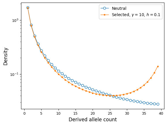
gamma = 10
h = 0.1

fs_yri_sel = moments.Spectrum.from_demes(
     ooa_model,
     sampled_demes=sampled_demes,
     sample_sizes=sample_sizes,
     gamma=gamma,
     h=h
)

We can compare the neutral and selected spectra:

# compare to neutral SFS for YRI
fig = plt.figure()
ax = plt.subplot(111)
ax.semilogy(fs_yri, "-o", ms=6, lw=1, mfc="w", label="Neutral");
ax.semilogy(fs_yri_sel, "-o", ms=3, lw=1,
    label=f"Selected, $\gamma={gamma}$, $h={h}$");
ax.set_ylabel("Density");
ax.set_xlabel("Derived allele count");
ax.legend();

We can gain more fine-grained control over variable selection and dominance in different populations by specifying gamma and h as dictionaries mapping population names to the coefficients. There can be as many different coefficient values as there are different demes in the demographic model. However, if a population is missing from the dictionary, it is assigned the default selection or dominance coefficient. In most cases the default values are \(\gamma = 0\) and \(h=1/2\), but these can be changed by specifying a _default value in the selection and dominance dictionaries.

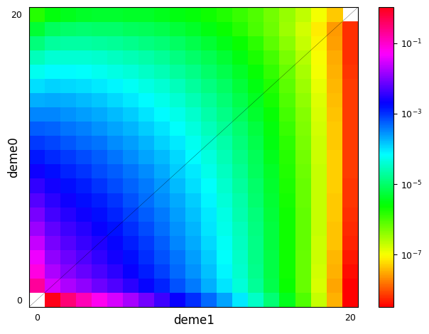
For example:

g = demes.load("data/im-parsing-example.yaml")
print(g)

gamma = {"anc": -10, "deme0": -10, "deme1": 5}
h = {"anc": 0.3, "deme0": 0.3, "deme1": 0.7}

fs = moments.Spectrum.from_demes(
    g,
    sampled_demes=["deme0", "deme1"],
    sample_sizes=[20, 20],
    gamma=gamma,
    h=h
)

moments.Plotting.plot_single_2d_sfs(fs)

description: A simple isolation-with-migration model
time_units: generations
generation_time: 1
demes:
- name: anc
  epochs:
  - {end_time: 1500, start_size: 10000}
- name: deme0
  ancestors: [anc]
  epochs:
  - {end_time: 0, start_size: 2000}
- name: deme1
  ancestors: [anc]
  epochs:
  - {end_time: 0, start_size: 20000}
migrations:
- demes: [deme0, deme1]
  rate: 0.0001

In the case that a demographic model has many populations but only a small subset have differing selection or dominance strengths, we can assign a default value different from \(s=0\) or \(h=1/2\). This is done by including a _default key in the dictionary (note the leading underscore, to minimize the chance that the default key conflicts with a named population in the demographic model). Taking the example above:

gamma = {"_default": -10, "deme1": 5}
h = {"_default": 0.3, "deme1": 0.7}

fs_defaults = moments.Spectrum.from_demes(
    g,
    sampled_demes=["deme0", "deme1"],
    sample_sizes=[20, 20],
    gamma=gamma,
    h=h
)

assert np.allclose(fs, fs_defaults)

Using Demes to infer demography

Above, we showed how to use moments and demes-based demographic models to compute expectations for static demographic models. That is, given a fixed demography we can compute expectations for the SFS or LD. We often want to optimize the parameters of a given demographic model to fit observations from data. The general idea is that we specify a parameterized model, compute the expected SFS under that model and its likelihood given the data, and then update the model parameters to improve the fit. Moments uses scipy’s optimization functions to perform optimization.

To run the inference, we need three items: 1) the data (SFS) to be fit, 2) a parameterized demographic model, and 3) a way to tell the optimization function which parameters to fit and any constraints on those parameters. We’ll assume you already have a data SFS with stored pop_ids. For example, the data could be a 3-dimensional SFS for the three sampled populations in the Out-of-Africa demographic model above, so that data.pop_ids = ["YRI", "CEU", "CHB"].

The second item is the demes-formatted demographic model, such as the model written above. In this model, the parameter values are the demographic event times, population sizes, and migration rates, and the YAML file specifies all fixed parameters and initial guesses for the parameters to be fit.

The third item is a separate YAML-formatted file that tells the optimization function the variable parameters that should be fit and any bounds and/or inequality constraints on the parameter values.

The options file

All parameters to be fit must be included under parameters in the option file. Any parameter that is not included here is assumed to be a fixed parameter, and it will remain the value given in the Demes graph. moments will read this YAML file into a dictionary using a YAML parser, so it needs to be valid and properly formatted YAML code.

The only required field in the “options” YAML is parameters. For each parameter to be fit, we must name that parameter, which can be any unique string, and we need to specify which values in the Demes graph correspond to that value (optionally, we can include a parameter description for our own sake). For example, to fit the bottleneck size in the Out-of-Africa model, our options file would look like:

parameters:
- name: N_B
  description: Bottleneck size for Eurasian populations
  values:
  - demes:
      OOA:
        epochs:
          0: start_size
  lower_bound: 100
  upper_bound: 100000

This specifies that the start size of the first (and only) epoch of the OOA deme in the Demes graph should be fit. We have also specified that the fit for this parameter should be bounded between 100 and 100,000.

The same parameter can affect multiple values in the Demes graph. For example, the size of the African population in the Out-of-Africa model is applied to both the AMH and the YRI demes. This simply requires adding additional keys in the values entry:

parameters:
- name: N_A
  description: Expansion size
    values:
    - demes:
        AMH:
          epochs:
            0: start_size
        YRI:
          epochs:
            0: start_size
  lower_bound: 100
  upper_bound: 100000

Migration rates can be specified to be fit as well. Note that the index of the migration is given, pointing to the migrations in the order they are specified in the demes file.

parameters:
- name: m_Af_Eu
  description: Symmetric migration rate between Afr and Eur populations
  upper_bound: 1e-3
  values:
  - migrations:
      1: rate

Note here that we have specified the upper bound to be 1e-3 (the units of the migration rate are parental migrant probabilities, typical in population genetics models). For any parameter, we can set the lower bound and upper bound as shown here. If they are not given, the lower bound defaults to 0 and the upper bound defaults to infinity.

Finally, we can also specify constraints on parameters. For example, if some event necessarily occurs before another, we should add that relationship to the list of constraints.

parameters:
- name: TA
  description: Time before present of ancestral expansion
  values:
  - demes:
      ancestral:
        epochs:
          0: end_time
- name: TB
  description: Time of YRI-OOA split
  values:
  - demes:
      AMH:
        epochs:
          0: end_time
- name: TF
  description: Time of CEU-CHB split
  values:
  - demes:
      OOA:
        epochs:
          0: end_time
constraints:
- params: [TA, TB]
  constraint: greater_than
- params: [TB, TF]
  constraint: greater_than

This specifies each of the event timings in the OOA model to be fit, and the constraints say that TA must be greater than TB, and TB must be greater than TF.

The inference function

To run optimization using the Demes modeul, we call moments.Demes.Inference.optimize. The first three required inputs to optimize are the Demes input graph, the parameter options, and the data, in that order.

Additional options can be passed to the optimization function using keyword arguments in the moments.Demes.Inference.optimize function. These include:

• maxiter: Maximum number of iterations to run optimization. Defaults to 1,000.

• perturb: Defaults to 0 (no perturbation of initial parameters). If greater than zero, it perturbs the initial parameters by up to perturb-fold. So if perturb is 1, initial parameters are randomly chosen from \([1/2\times p_0, 2\times p_0]\). Larger values result in stronger perturbation of initial guesses.

• verbose: Defaults to 0. If greater than zero, it prints an update to the specified output_stream (which defaults to sys.stdout) every verbose iterations.

• uL: Defaults to None. If given, this is the product of the per-base mutation rate and the length of the callable genome used to compile the data SFS. If we don’t give this scaled mutation rate, we optimize with theta as a free parameter. Otherwise, we optimize with theta given by \(\theta=4 \times N_e \times uL\), and \(N_e\) is taken to be the size of the root/ancestral deme (for which the size can be a either be a fixed parameter or a parameter to be fit!).

• log: Defaults to True. If True, optimize the log of the parameters.

• method: The optimization method to use, currently with the options “fmin” (Nelder-Mead), “powell”, or “lbfgsb”. Defaults to “fmin”.

• fit_ancestral_misid: Defaults to False, and cannot be used with a folded SFS. For an unfolded SFS, the ancestral state may be misidentified, resulting in a distortion of the SFS. We can account for that distortion by fitting a parameter that accounts for some fraction of mis-labeled ancestral states.

• misid_guess: Used with fit_ancestral_misid, as the initial ancestral misidentification parameter guess. Defaults to 0.02.

• output_stream: Defaults to sys.stdout.

• output: Defaults to None, in which case the result is printed to the output_stream. If given, write the optimized Demes graph in YAML format to the given path/filename.

• overwrite: Defaults to False. If True, we overwrite any file with the path/filename given by output.

Single-population inference example

To demonstrate, we’ll fit a simple single-population demographic model to the synonymous variant SFS in the Mende (MSL) from the Thousand Genomes data. The data for this population is stored in the docs/data directory. We previous parsed all coding variation and used a mutation model to estimate \(u\times L\).

We can either fold the frequency spectrum, which is useful when we do not know the ancestral states of mutations. Alternatively, we can fit with the unfolded spectrum, and if we suspect that some proportion of SNPs have their ancestral state misidentified, we can additionally fit a parameter that corrects for this uncertainty. We’ll take the second approach here, and fit the unfolded spectrum.

import moments
import pickle

all_data = pickle.load(open("./data/msl_data.bp", "rb"))
data = all_data["spectra"]["syn"]
data.pop_ids = ["MSL"]
uL = all_data["rates"]["syn"]
print("scaled mutation rate (u_syn * L):", uL)

# project down to a smaller sample size, for illustration purposes
data = data.project([30])

scaled mutation rate (u_syn * L): 0.14419746897690008

We’ll fit a demographic model that includes an ancient expansion and a more recent exponential growth. This initial model is stored in the docs/data directory as well.

The YAML specification of this model is

description: A single-population model to be fit to the MSL data. Initial guesses
  are given as parameters in the model.
time_units: years
generation_time: 29
demes:
- name: MSL
  epochs:
  - end_time: 350000
    start_size: 10000
  - end_time: 20000
    start_size: 25000
  - end_time: 0
    end_size: 60000

And we can specify that we want to fit the times of the size changes, and all population sizes. (Note that if we did not have an estimate for the mutation rate, we would not fit the ancestral size.)

parameters:
- name: T1
  description: Time before present of ancestral expansion
  values:
  - demes:
      MSL:
        epochs:
          0: end_time
- name: T2
  description: Time before present of start of exponential growth.
  values:
  - demes:
      MSL:
        epochs:
          1: end_time
- name: Ne
  description: Effective (ancestral/root) size
  values:
  - demes:
      MSL:
        epochs:
          0: start_size
- name: NA
  description: Ancestral expansion size
  values:
  - demes:
      MSL:
        epochs:
          1: start_size
- name: NF
  description: Final population size
  values:
  - demes:
      MSL:
        epochs:
          2: end_size
constraints:
- params: [T1, T2]
  constraint: greater_than

deme_graph = "./data/msl_initial_model.yaml"
options = "./data/msl_options.yaml"

And now we can run the inference:

output = "./data/msl_best_fit_model.yaml"
ret = moments.Demes.Inference.optimize(
    deme_graph,
    options,
    data,
    uL=uL,
    fit_ancestral_misid=True,
    misid_guess=0.01,
    method="lbfgsb",
    output=output,
    overwrite=True
)
param_names, opt_params, LL = ret
print("Log-likelihood:", -LL)
print("Best fit parameters")
for n, p in zip(param_names, opt_params):
    print(f"{n}\t{p:.3}")

Log-likelihood: -126.08823318048917
Best fit parameters
T1	4.38e+05
T2	2.2e+04
Ne	1.09e+04
NA	2.5e+04
NF	6.6e+04
p_misid	0.026

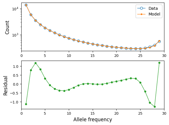
Printed above are the best fit parameters for this model, including the ancestral misidentification rate for synonymous variants in the Mende sample. Parameters in this fit are scaled by our estimate of the total mutation rate of synonymous variants (uL), which allows us to infer the ancestral \(N_e\). Below, we plot the results and then compute confidence intervals for this fit.

Plotting the results

We can see how well our best fit model fits the data, using moments plotting features:

fs = moments.Spectrum.from_demes(output, samples={"MSL": data.sample_sizes})
fs = moments.Misc.flip_ancestral_misid(fs, opt_params[-1])
moments.Plotting.plot_1d_comp_multinom(fs, data)

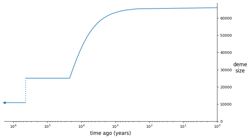
And we can illustrate the best fit model using demesdraw:

import demes, demesdraw
opt_model = demes.load(output)
demesdraw.size_history(opt_model, invert_x=True, log_time=True);

Computing confidence intervals

Using the output YAML from moments.Demes.Inference.optimize(), we compute confidence intervals using moments.Demes.Inference.uncerts(). This function takes the output Demes graph from the optimization, the same parameter options file, and the same data used in inference. These need to be consistent between the optimization and uncertainty computation. If we specified the mutation rate or inferred an ancestral misidentification parameter, those must also be provided.

The additional options to uncerts() are

• bootstraps: Defaults to None, in which case we use the FIM approach.

• uL: The scaled mutation rate, if used in the optimization. (See above for details.)

• log: Defaults to False. If True, we assume a log-normal distribution of parameters. Returned values are then the standard deviations of the logs of the parameter values, which can be interpreted as relative parameter uncertainties.

• eps: The relative step size to use when numerically computing derivatives to estimate the curvature of the likelihood function at the inferred best-fit parameters.

• method: Defaults to “FIM”, which uses the Fisher information matrix. We can also use the Godambe information matrix, which uses bootstrap replicates to account for non-independence between linked SNPs. This uses methods developed by Alec Coffman in Ryan Gutenkunst’s group, described in [Coffman2016].

• fit_ancestral_misid: If the ancestral misid was fit, this should be set to True.

• misid_fit: The fit misidentification parameter, if it was fit.

• output_stream: Defaults to sys.stdout.

In our example using the Mende data above, we’ll use the FIM method compute confidence intervals:

std_err = moments.Demes.Inference.uncerts(
    output,
    options,
    data,
    uL=uL,
    fit_ancestral_misid=True,
    misid_fit=opt_params[-1],
)

print("95% CIs")
print("param\t\t2.5%\t\t97.5%")
for n, p, e in zip(param_names, opt_params, std_err):
    print(f"{n}\t{p - 1.96 * e:-12g}\t{p + 1.96 * e:-13g}")

95% CIs
param		2.5%		97.5%
T1	      378253	       497820
T2	     10528.9	      33528.2
Ne	     10387.3	      11316.9
NA	     23521.2	      26539.5
NF	     41670.7	      90313.3
p_misid	   0.0228469	    0.0291068

To compute standard errors that account for non-independence between SNPs, we would use method="GIM" and include a list of bootstrap replicate spectra that we pass to bootstraps.

Two-population inference and uncertainty example

Here, we’ll simulate a demographic model using msprime. In this example, we’ll simulate many regions of varying length and mutation rates, from which we compute uL and estimate confidences using the GIM method, which requires bootstrapped datasets of the SFS and associated scaled mutation rates.

First, we’ll simulate data under this two-population model:

g = demes.load("./data/two-deme-example.yaml")
print(g)

time_units: generations
generation_time: 1
demes:
- name: anc
  epochs:
  - {end_time: 2000, start_size: 8500}
- name: A
  ancestors: [anc]
  epochs:
  - {end_time: 0, start_size: 700, end_size: 11000}
- name: B
  ancestors: [anc]
  epochs:
  - {end_time: 0, start_size: 17500}
migrations:
- demes: [A, B]
  rate: 0.0015

import msprime

demog = msprime.Demography.from_demes(g)

num_regions = 200
# Lengths between 75 and 125 kb
Ls = np.random.randint(75000, 125000, 200)
# Mutation rates between 1e-8 and 2e-8
us = 1e-8 + 1e-8 * np.random.rand(200)

# Total mutation rate
uL = np.sum(us * Ls)

# Simulate and store allele frequency data (summed and by region)
ns = [20, 20]
region_data = {}
data = moments.Spectrum(np.zeros((ns[0] + 1, ns[1] + 1)))
data.pop_ids = ["A", "B"]
# sample_sets are required to get the SFS from the tree sequences
sample_sets = (range(20), range(20, 40))

for i, (u, L) in enumerate(zip(us, Ls)):
    ts = msprime.sim_ancestry(
        {"A": ns[0] // 2, "B": ns[1] // 2},
        demography=demog,
        recombination_rate=1e-8,
        sequence_length=L,
    )
    ts = msprime.sim_mutations(ts, rate=u)
    SFS = ts.allele_frequency_spectrum(
        sample_sets=sample_sets, span_normalise=False, polarised=True)
    region_data[i] = {"uL": u * L, "SFS": SFS}
    data += SFS

print("Simulated data. FST =", data.Fst())

Simulated data. FST = 0.03488586466502664

With this simulated data, we can now re-infer the model, using the following options:

parameters:
- name: T
  description: Ancestral split time
  values:
  - demes:
      anc:
        epochs:
          0: end_time
- name: Ne
  description: Ancestral effective population size
  values:
  - demes:
      anc:
        epochs:
          0: start_size
- name: NA0
  description: Initial population size of A
  values:
  - demes:
      A:
        epochs:
          0: start_size
- name: NA
  description: Final population size of A
  values:
  - demes:
      A:
        epochs:
          0: end_size
- name: NB
  description: B population size  
  values:
  - demes:
      B:
        epochs:
          0: start_size
- name: M
  description: migration rate between A and B
  values:
  - migrations:
      0: rate
  upper_bound: 1

deme_graph = "./data/two-deme-example.yaml"
options = "./data/two-deme-example-options.yaml"
output = "./data/two-deme-example-best-fit.yaml"

ret = moments.Demes.Inference.optimize(
    deme_graph,
    options,
    data,
    uL=uL,
    perturb=1,
    output=output,
    overwrite=True
)

Printing the results of this inference run:

param_names, opt_params, LL = ret
print("Log-likelihood:", -LL)
print("Best fit parameters")
for n, p in zip(param_names, opt_params):
    print(f"{n}\t{p:.3}")

Log-likelihood: -1296.725088604149
Best fit parameters
T	1.52e+03
Ne	8.61e+03
NA0	5.74e+02
NA	2.05e+04
NB	1.46e+04
M	0.00115

To compute confidence intervals using the Godambe method, we need generate bootstrap replicates of the data (and scaled mutation rate, if specified in the optimization).

bootstraps = []
bootstraps_uL = []
for _ in range(len(region_data)):
    choices = np.random.choice(range(200), 200, replace=True)
    bootstraps.append(
        moments.Spectrum(sum([region_data[c]["SFS"] for c in choices])))
    bootstraps_uL.append(sum([region_data[c]["uL"] for c in choices]))

Computing the uncertainties using GIM requires passing the bootstrapped data:

std_err = moments.Demes.Inference.uncerts(
    output,
    options,
    data,
    bootstraps=bootstraps,
    uL=uL,
    bootstraps_uL=bootstraps_uL,
    method="GIM",
)

print("Standard errors:")
print("param\t\topt\t\tstderr")
for n, p, e in zip(param_names, opt_params, std_err):
    print(f"{n}\t{p:-11g}\t{e:-14g}")

Standard errors:
param		opt		stderr
T	     1515.2	       183.786
Ne	    8607.87	       179.118
NA0	    573.705	       84.0684
NA	      20466	        5675.2
NB	    14610.3	       1994.22
M	 0.00115135	   0.000150782

References

[Gutenkunst2009]

Gutenkunst, Ryan N., et al. “Inferring the joint demographic history of multiple populations from multidimensional SNP frequency data.” PLoS genet 5.10 (2009): e1000695.

[Ragsdale2020]

Ragsdale, Aaron P., et al. “Lessons learned from bugs in models of human history.” The American Journal of Human Genetics 107.4 (2020): 583-588.