Parsing LD statistics
As described in the multi-population LD section, we are interested in \(\sigma_d^2\)-type statistics, which is the ratio of expectations of \(D^2\) and \(\pi_2 = p(1-p)q(1-q)\). Again, \(p\) and \(q\) are the allele frequencies at the left and right loci.
To estimate these statistics from data, we take the average of each LD statistic over all pairs of observed (biallelic) SNPs at a given recombination distance, and then divide by the observed \(\pi_2\) in one of the populations (the “normalizing” population). As described below, we also use a block bootstrapping approach to estimate variances and covariances of observed statistics at each recombination distance, which is used in inference and computing confidence intervals.
Binned LD decay
To estimate LD decay curves from the data, we bin all pairs of observed SNPs by recombination distance. While we can bin by physical distance (bps) separating SNPs, genetic maps are non-uniform and physical distance does not perfectly correlate with genetic distance at small scales. If we have a recombination map available, it is preferable to compute and compare statistics using that map.
Recombination rate bins are defined by bin edges, which is a list or array with length equal to the number of desired bins plus one. Bin edges should be monotonically increasing, and are thus adjacent without gaps between bins. Thus, bins are defined as semi-open intervals:
import moments.LD
import numpy as np

bin_edges = np.array([0, 1e-6, 1e-5, 1e-4])
print("Bins:")
for b_l, b_r in zip(bin_edges[:-1], bin_edges[1:]):
    print(f"[{b_l}, {b_r})")
Bins:
[0.0, 1e-06)
[1e-06, 1e-05)
[1e-05, 0.0001)
There are a few considerations to keep in mind. In practice, very short distances can be problematic, because “non-standard” evolutionary processes can distort allele frequency correlations for tightly linked loci. For example, our evolutionary model does not include multi-nucleotide mutations [Harris2014] or gene conversion [Ardlie2001], both of which operate at short distances.
Thus, when working with real data we recommend omitting bins of very short recombination distances. In practice, we typically drop bins with length less than \(r=5\times 10^{-6}\), which corresponds to roughly a few hundred bp on average in humans.
Parsing from a VCF
The primary function of the Parsing module is computing LD statistics from an
input VCF. There are a number of options available, but the primary inputs are
the path to the VCF file and the bins of distances separating loci. Typically, we
work in recombination distance, in which case a recombination map is also required.
If we do not have a recombination map available, we can bin by base pair distances
instead.
The function moments.LD.Parsing.compute_ld_statistics returns a dictionary with
the bins, returned statistics, populations, and sums of each statistic over the
provided bins. For example:
r_bins = np.logspace(-6, -3, 7)
ld_stats = moments.LD.Parsing.compute_ld_statistics(
    vcf_path, r_bins=r_bins, rec_map_file=map_path)
Using a recombination map
The input recombination map is specified as a text file, with the first column giving
positions along the chromosome and additional column(s) defining the cumulative map(s),
typically in units of cM. The header line is “Pos Map1 Map2 (etc)”, and we can use
any map in the file by specifying the map_name. If no map name is given, or the
specified map name does not match a genetic map in the header, we use the map in the
first column.
Typically, maps are given in units of centi-Morgans, and the default behavior is to
assume cM units. If the map is given in units of Morgans, we need to set cM=False.
Populations and pop-file
We often have data from more than one population, so we need to be able to specify which samples in the VCF correspond to which populations. This is handled by passing a file that assigns each sample to a population. For example, the population file is written as
sample  pop
sid_0   pop_A
sid_1   pop_B
sid_2   pop_A
sid_3   pop_A
sid_4   pop_B
...
Then to include the population information in the function, we also pass a list of the populations to compute statistics for. Samples from omitted populations are dropped from the data.
pops = ["pop_A", "pop_B"]
ld_stats = ld_stats = moments.LD.Parsing.compute_ld_statistics(
    vcf_path,
    r_bins=r_bins,
    rec_map_file=map_path,
    pop_file=pop_file_path,
    pops=pops
)
Masking and using bed files
If there are multiple chromosomes or contigs included in the VCF, we specify
which chromosome to compute statistics for by setting the chromosome flag.
We can also subset a chromosome by including a bed file, which will filter out
all SNPs that fall outside the region intervals given in the bed file. Bed files
have the format {chrom}\t{left_pos}\t{right_pos}, which defines a semi-open
interval. The path to the bed file is provided with the bed_file argument.
Computing a subset of statistics
Sometimes we may wish to only compute a subset of possible LD statistics. By
default, the parsing function computes all statistics possible for the number
of populations provided. Instead, we can specify the stats_to_compute, which
is a list (of length 2) of lists. The first list are the LD statistics to return,
and the second list has the heterozygosity statistics to return. Statistic names
follow the convention in moments.LD.Util.moment_names(num_pops), and should
be formatted accordingly.
Phased vs unphased data
We can compute LD statistics from either phased or unphased data. The default
behavior is to assume that phasing is unknown, and use_genotypes is
True by default. If we want to compute LD using phased data, we set
use_genotypes=False, and parsing uses phased haplotypes instead. In
general, phasing errors can bias LD statistics, sometimes significantly, and
using genotypes instead of haplotypes only slightly increases uncertainty in
most cases. Therefore, we usually recommend leaving use_genotypes=True.
Computing averages and covariances over regions
From moments.LD.Parsing.compute_ld_statistics(), we get LD statistic sums
from the regions in a VCF, perhaps constrained by a bed file. Our strategy is
to divide our data into some large number of roughly equally sized chunks, for
example 500 regions across all 22 autosomes in human data. We then compute LD
statistics independently for each region (it helps to parallelize that step,
using a compute cluster). From those outputs, we can then compute average
statistics genome-wide, as well as covariances of statistics within each bin.
Those covariances are needed to be able to compute likelihoods and run
optimization.
The outputs of compute_ld_statistics are compiled in a dictionary, where
the keys are unique region identifiers, and items the outputs of that function.
For example:
region_stats = {
    0: moments.LD.Parsing.compute_ld_statistics(VCF, bed_file="region_0.bed", ...),
    1: moments.LD.Parsing.compute_ld_statistics(VCF, bed_file="region_1.bed", ...),
    2: moments.LD.Parsing.compute_ld_statistics(VCF, bed_file="region_2.bed", ...),
    ...
}
Mean and variance-covariance matrices are computed by calling
bootstrap_data, passing the region statistics dictionary, and optionally
the index of the population to normalize \(\sigma_d^2\) statistics by. By
default, the normalizing population is the first (index 0).
mv = moments.LD.Parsing.bootstrap_data(region_stats)
mv contains the bins, statistics, and populations, as well as lists of mean
statistics and variance-covariance matrices. This data can then be directly
compared to model expectations and used in inference.
Example
Using msprime
[Kelleher2016], we’ll simulate some data under an isolation-with-migration
(IM) model and then compute LD and heterozygosity statistics using the
LD.Parsing methods. First, the simulation will use the
demes-msprime interface, which are then written as a VCF.
The YAML-file specifying the model is
description: A simple isolation-with-migration model
time_units: generations
demes:
- name: anc
  epochs: [{start_size: 10000, end_time: 1500}]
- name: deme0
  ancestors: [anc]
  epochs: [{start_size: 2000}]
- name: deme1
  ancestors: [anc]
  epochs: [{start_size: 20000}]
migrations:
- demes: [deme0, deme1]
  rate: 1e-4
And we use msprime to simulate 1Mb of data, using a constant recombination and mutation rate.
import msprime
import demes
import os

# set up simulation parameters
L = 1e6
u = r = 1.5e-8
n = 10

g = demes.load("data/im-parsing-example.yaml")
demog = msprime.Demography.from_demes(g)

trees = msprime.sim_ancestry(
    {"deme0": n, "deme1": n},
    demography=demog,
    sequence_length=L,
    recombination_rate=r,
    random_seed=321,
)

trees = msprime.sim_mutations(trees, rate=u, random_seed=123)

with open("data/im-parsing-example.vcf", "w+") as fout:
    trees.write_vcf(fout)
This simulation had 10 diploid individuals per population, and
msprime/tskit writes their IDs as tsk_0, tsk_1, etc:
##fileformat=VCFv4.2
##source=tskit 0.3.5
##FILTER=<ID=PASS,Description="All filters passed">
##contig=<ID=1,length=1000000>
##FORMAT=<ID=GT,Number=1,Type=String,Description="Genotype">
#CHROM	POS	ID	REF	ALT	QUAL	FILTER	INFO	FORMAT	tsk_0	tsk_1	tsk_2	tsk_3	tsk_4	tsk_5	tsk_6	tsk_7	tsk_8	tsk_9	tsk_10	tsk_11	tsk_12	tsk_13	tsk_14	tsk_15	tsk_16	tsk_17	tsk_18	tsk_19
1	221	.	A	T	.	PASS	.	GT	1|1	1|0	1|1	1|1	0|1	0|1	0|0	1|1	0|1	1|1	1|1	1|1	1|1	1|1	1|1	1|1	1|1	1|1	1|1	1|1
1	966	.	A	C	.	PASS	.	GT	0|0	0|0	0|0	0|0	0|0	0|0	0|0	1|1	0|0	0|0	0|0	0|0	0|1	0|0	0|0	0|0	0|0	0|0	0|1	1|0
1	1082	.	G	A	.	PASS	.	GT	0|0	0|1	0|0	0|0	1|0	1|0	1|1	0|0	1|0	0|0	0|0	0|0	0|0	0|0	0|0	0|0	0|0	0|0	0|0	0|0
1	1133	.	G	T	.	PASS	.	GT	0|0	0|1	0|0	0|0	1|0	1|0	1|1	0|0	1|0	0|0	0|0	0|0	0|0	0|0	0|0	0|0	0|0	0|0	0|0	0|0
To parse this data, we need the file that maps samples to populations and the recombination map file (the total map length is found by \(1 \times 10^{6} \text{ bp} \times 1.5 \times 10^{-8} \text{ M/bp} \times 100 \text{ cM/M}\)):
sample  pop
tsk_0   deme0
tsk_1   deme0
tsk_2   deme0
tsk_3   deme0
tsk_4   deme0
tsk_5   deme0
tsk_6   deme0
tsk_7   deme0
tsk_8   deme0
tsk_9   deme0
tsk_10  deme1
tsk_11  deme1
tsk_12  deme1
tsk_13  deme1
tsk_14  deme1
tsk_15  deme1
tsk_16  deme1
tsk_17  deme1
tsk_18  deme1
tsk_19  deme1
Pos Map(cM)
0   0
1000000 1.5
With all this, we can now compute LD based on recombination distance bins:
r_bins = np.array(
    [0, 1e-6, 2e-6, 5e-6, 1e-5, 2e-5, 5e-5, 1e-4, 2e-4, 5e-4, 1e-3]
)

vcf_file = "data/im-parsing-example.vcf"
map_file = "data/im-parsing-example.map.txt"
pop_file = "data/im-parsing-example.samples.pops.txt"
pops = ["deme0", "deme1"]
ld_stats = moments.LD.Parsing.compute_ld_statistics(
    vcf_file,
    rec_map_file=map_file,
    pop_file=pop_file,
    pops=["deme0", "deme1"],
    r_bins=r_bins,
    report=False,
)
The output, ld_stats, is a dictionary with the keys bins, stats,
pops, and sums. To get the average statistics over multiple regions
(here, we only have a single region that we simulated), we use
means_from_region_data:
means = moments.LD.Parsing.means_from_region_data(
    {0: ld_stats}, ld_stats["stats"], norm_idx=0
)
This provides \(\sigma_d^2\)-type statistics relative to pi_2 in
deme0, and relative heterozygosities (also relative to deme0).
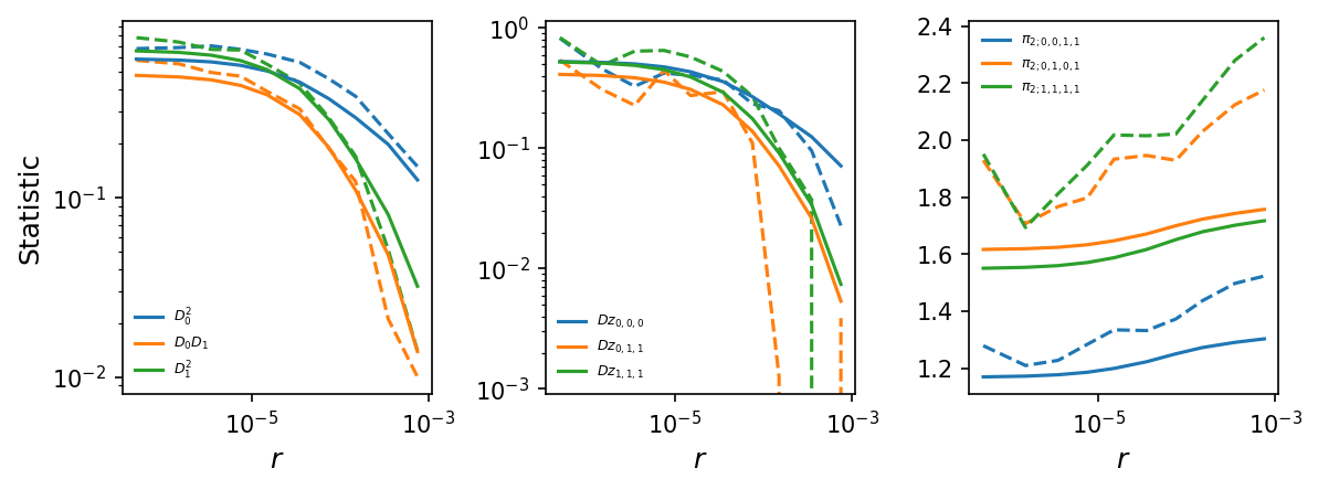
These statistics were computed from only a single relatively small region,
so they will be quite noisy. But we can still compare to expectations under
the input IM demographic model.
import demes
g = demes.load("data/im-parsing-example.yaml")

y = moments.Demes.LD(
    g,
    sampled_demes=["deme0", "deme1"],
    rho=4 * g["anc"].epochs[0].start_size * r_bins,
)

# stats are computed at the bin edges - average to get midpoint estimates
y = moments.LD.LDstats(
    [(y_l + y_r) / 2 for y_l, y_r in zip(y[:-2], y[1:-1])] + [y[-1]],
    num_pops=y.num_pops,
    pop_ids=y.pop_ids,
)
y = moments.LD.Inference.sigmaD2(y)

# plot LD decay curves for some statistics
moments.LD.Plotting.plot_ld_curves_comp(
    y,
    means[:-1],
    [],
    rs=r_bins,
    stats_to_plot=[
        ["DD_0_0", "DD_0_1", "DD_1_1"],
        ["Dz_0_0_0", "Dz_0_1_1", "Dz_1_1_1"],
        ["pi2_0_0_1_1", "pi2_0_1_0_1", "pi2_1_1_1_1"]
    ],
    labels=[[r"$D_0^2$", r"$D_0 D_1$", r"$D_1^2$"],
        [r"$Dz_{0,0,0}$", r"$Dz_{0,1,1}$", r"$Dz_{1,1,1}$"],
        [r"$\pi_{2;0,0,1,1}$", r"$\pi_{2;0,1,0,1}$", r"$\pi_{2;1,1,1,1}$"]
    ],
    plot_vcs=False,
    fig_size=(8, 3),
    show=True,
)
Bootstrapping over multiple regions
Normally, we’ll want more data than from a single 1Mb region to compute
averages and variances of statistics. Using the same approach as the above
example, ld_stats for 100 replicates we computed (see example in the
moments repository here). From
this, each replicate set of statistics were placed in a dictionary, as
rep_stats = {0: ld_stats_0, 1: ld_stats_1, ..., 99: ld_stats_99}. This
dictionary can then be used to compute means and covariances of statistics.
mv = moments.LD.Parsing.bootstrap_data(ld_stats)
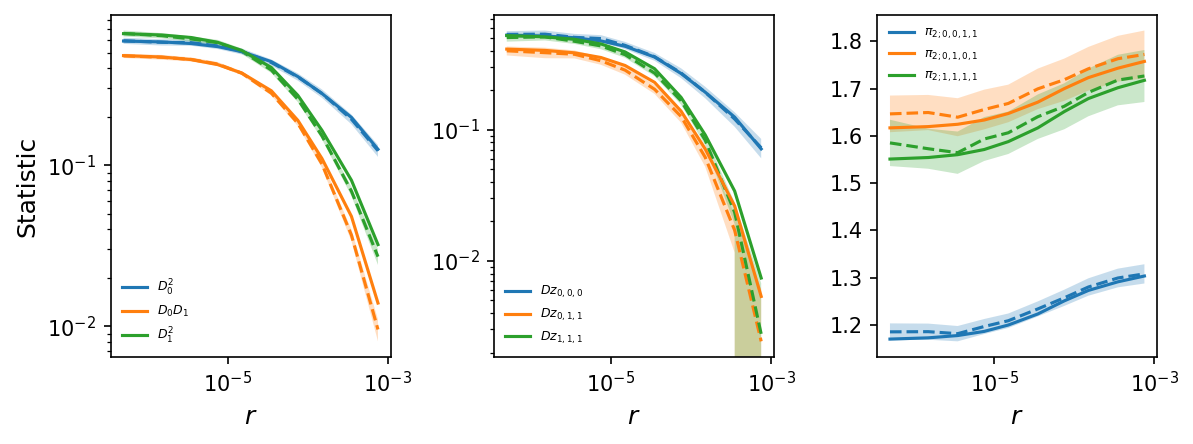
By simulating more data, the LD decay curves are much less noisy, and by simulating multiple replicates, we also compute the variance-covariance matrices for each bin and can include standard errors in the plots.
# plot LD decay curves for some statistics
moments.LD.Plotting.plot_ld_curves_comp(
    y,
    mv["means"][:-1],
    mv["varcovs"][:-1],
    rs=r_bins,
    stats_to_plot=[
        ["DD_0_0", "DD_0_1", "DD_1_1"],
        ["Dz_0_0_0", "Dz_0_1_1", "Dz_1_1_1"],
        ["pi2_0_0_1_1", "pi2_0_1_0_1", "pi2_1_1_1_1"]
    ],
    labels=[[r"$D_0^2$", r"$D_0 D_1$", r"$D_1^2$"],
        [r"$Dz_{0,0,0}$", r"$Dz_{0,1,1}$", r"$Dz_{1,1,1}$"],
        [r"$\pi_{2;0,0,1,1}$", r"$\pi_{2;0,1,0,1}$", r"$\pi_{2;1,1,1,1}$"]
    ],
    plot_vcs=True,
    fig_size=(8, 3),
    show=True,
)
Note
The means-covariances data is required for inference using LD statistics.
In Inferring demography with LD, we’ll use the
same mv data dictionary to refit the IM model as an example.
LD statistics in genotype blocks
moments.LD.Parsing also includes some functions for computing LD from
genotype (or haplotype) blocks. Genotype blocks are arrays of shape
\(L\times n\), where L is the number of loci and n is the sample size.
We assume a single population, and so we compute \(D^2\), \(Dz\),
\(\pi_2\), and \(D\), either pairwise or averaged over all pairwise
comparisons.
If we have a genotype matrix containing n diploid samples, genotypes are
coded as 0, 1, and 2, and we set genotypes=True. If we have a haplotype
matrix with data from n haploid copies, genotypes are coded as 0 and 1 only,
and we set genotypes=False.
For example, given a single genotype matrix, we compute all pairwise statistics and average statistics as shown below:
L = 10
n = 5
G = np.random.randint(3, size=L * n).reshape(L, n)

# all pairwise comparisons:
D2_pw, Dz_pw, pi2_pw, D_pw = moments.LD.Parsing.compute_pairwise_stats(G)

# averages:
D2_ave, Dz_ave, pi2_ave, D_ave = moments.LD.Parsing.compute_average_stats(G)
Similarly, we can compute the pairwise or average statistics between two genotype matrices. The matrices can have differing number of loci, but they must have the same number of samples, as the genotype matrices are assumed to come from different regions within the same samples.
L2 = 12
n = 5

G2 = np.random.randint(3, size=L2 * n).reshape(L2, n)

# all pairwise comparisons:
D2_pw, Dz_pw, pi2_pw, D_pw = moments.LD.Parsing.compute_pairwise_stats_between(G, G2)

# averages:
D2_ave, Dz_ave, pi2_ave, D_ave = moments.LD.Parsing.compute_average_stats_between(G, G2)
Note
Computing LD in genotype blocks uses C-extensions that are not built by
default, so are only available if these are built when compiling the
C-extensions. In order to use these methods, we need to build these
extensions using the --ld_extensions flag, as python setup.py
build_ext --ld_extensions -i.
References
Ardlie, Kristin, et al. “Lower-than-expected linkage disequilibrium between tightly linked markers in humans suggests a role for gene conversion.” The American Journal of Human Genetics 69.3 (2001): 582-589.
Harris, Kelley, and Rasmus Nielsen. “Error-prone polymerase activity causes multinucleotide mutations in humans.” Genome research 24.9 (2014): 1445-1454.
Kelleher, Jerome, Alison M. Etheridge, and Gilean McVean. “Efficient coalescent simulation and genealogical analysis for large sample sizes.” PLoS computational biology 12.5 (2016): e1004842.