Selection at two loci
By Aaron Ragsdale, January 2021.
Note
This module has not been completed - I’ve placed to-dos where content is incoming. If you find an error here, or find some aspects confusing, please don’t hesitate to get in touch or open an issue. Thanks!
Most users of moments will be most interested in computing the single-site SFS and
comparing it to data. However, moments can do much more, such as computing expectations
for LD under complex demography, or triallelic or two-locus frequency spectra. Here, we’ll
explore what we can do with the two-locus methods available in moments.TwoLocus.
import moments.TwoLocus
import numpy as np
import matplotlib.pylab as plt
import pickle, gzip
The two-locus allele frequency spectrum
Similar to the single-site SFS, the two-locus frequency spectrum stores the number (or density) of pairs of loci with given two-locus haplotype counts. Suppose the left locus permits alleles A/a and the right locus permits B/b, so that there are four possible haplotypes: (AB, Ab, aB, and ab). In a sample size of n haploid samples, we observe some number of each haplotype, \(n_{AB} + n_{Ab} + n_{aB} + n_{ab} = n\). The two-locus frequency spectrum stores the observed number of pairs of loci with each possible sampling configuration, so that \(\Psi_n(i, j, k)\) is the number (or density) of pairs of loci with i type AB, j type Ab, and k type aB.
moments.TwoLocus lets us compute the expectation of \(\Psi_n\) for
single-population demographic scenarios, allowing for population size changes over time,
as well as arbitrary recombination distance separating the two loci and selection at
one or both loci. While moments.TwoLocus has a reversible mutation model implemented,
here we’ll focus on the infinite sites model (ISM), under the assumption that
\(N_e \mu \ll 1\) at both loci.
Below, we’ll walk through how to compute the sampling distribution for two-locus haplotypes for a given sample size, describe its relationship to common measures of linkage disequilibrium (LD), and explore how recombination, demography, and selection interacts to alter expected patterns of LD. In particular, we’ll focus on a few different models of selection, dominance, and epistasic interactions between loci, and ask under what conditions those patterns are expected to differ or to be confounded.
Citing this work
Demographic inference using a diffusion approximation-based solution for \(\Psi_n\) was introduced in [Ragsdale_Gutenkunst]. The moments-based method, which is implemented here, was described in [Ragsdale_Gravel].
Two-locus haplotype distribution under neutrality
A quick comment on computational efficiency
The frequency spectrum \(\Psi_n\) is displayed as a 3-dimensional array in moments, and the size grows quite quickly in the sample size \(n\). (The number of frequency bins is \(\frac{1}{6}(n+1)(n+2)(n+3)\), so it grows as \(n^3\).) Thus, solving for \(\Psi\) gets quite expensive for large sample sizes.
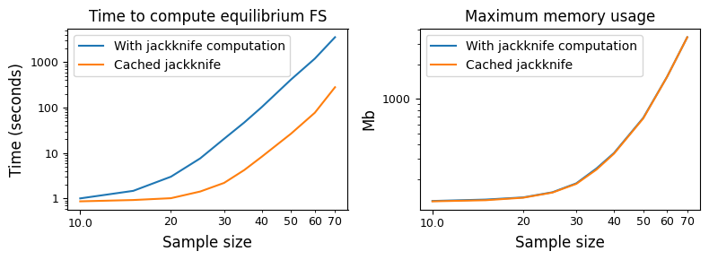
Here, we see the time needed to compute the equilibrium frequency spectrum for a given sample size. Recombination requires computing a jackknife operator for approximate moment closure, which gets expensive for large sample sizes. However, we can cache and reuse this jackknife matrix (the default behavior), so that much of the computational time is saved from having to recompute that large matrix. However, we see that simply computing the steady-state solution still gets quite expensive as the sample sizes increase.
Below, we’ll see that for non-zero recombination (as well as selection) our accuracy improves as we increase the sample size. For this reason, we’ve pre-computed and cached results throughout this page, and the code blocks give examples of how those results were created.
Two neutral loci
The moments.TwoLocus solution for the neutral frequency spectrum without recombination
(\(\rho = 4 N_e r = 0\)) is exact, while \(\rho > 0\) and selection require a
moment-closure approximation. This approximation grows more accurate for larger \(n\).
To get familiar with some common two-locus statistics (either summaries of \(\Psi_n\) and \(\Psi\) itself), we can compare to some classical results, such as the expectation for \(\sigma_d^2 = \frac{\mathbb{E}[D^2]}{\mathbb{E}[p(1-p)q(1-q)]}\), where D is the standard covariance measure of LD, and p and q are allele frequencies at the left and right loci, respectively [Ohta]:
rho = 0
n = 10
Psi = moments.TwoLocus.Demographics.equilibrium(n, rho=rho)
sigma_d2 = Psi.D2() / Psi.pi2()
print(r"moments.TwoLocus $\sigma_d^2$, $r=0$:", sigma_d2)
print(r"Ohta and Kimura expectation, $r=0$:", 5 / 11)
moments.TwoLocus $\sigma_d^2$, $r=0$: 0.4545454545454553
Ohta and Kimura expectation, $r=0$: 0.45454545454545453
And we can plot the LD-decay curve for \(\sigma_d^2\) for a range of recombination rates and a few different sample sizes, and compare to [Ohta]’s expectation, which is \(\sigma_d^2 = \frac{5 + \frac{1}{2}\rho}{11 + \frac{13}{2}\rho + \frac{1}{2}\rho^2}\):
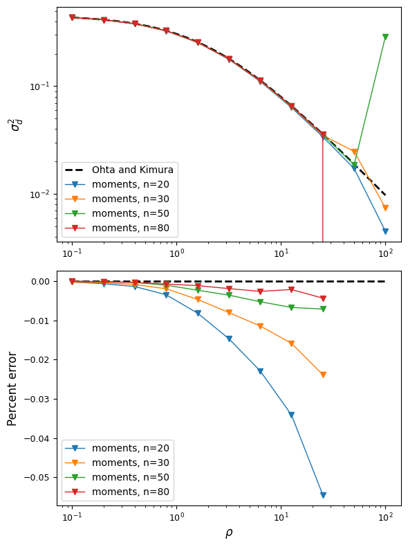
The moments approximation breaks down for recombination rates around \(\rho\approx50\)
but is very accurate for lower recombination rates, and this accuracy increases with the
sample size. To be safe, we can assume that numerical error starts to creep
in around \(rho\approx25\), which for human parameters, is very roughly 50 or 100kb.
So we’re limited to looking at LD in relatively shorter regions. For higher recombination
rates, we can turn to moments.LD, which lets us model multiple populations, but
is restricted to neutral loci and low-order statistics.
The statistics \(\mathbb{E}[D^2]\) and \(\mathbb{E}[p(1-p)q(1-q)]\) are low-order summaries of the full sampling distribution, similar to how heterozygosity or Tajima’s D are low-order summaries of the single-site SFS. We can visualize some features of the full two-locus haplotype frequency distribution instead, following Figure 1 in Hudson’s classical paper on the two-locus sampling distribution [Hudson]. Here, we’ll look at a slice in the 3-dimensional distribution: if we observe \(n_A\) samples carrying A at the left locus, and \(n_B\) carrying B at the right locus, what is the probability that we observe n_{AB} haplotypes with A and B coupled in the same sample? This marginal distribution will depend on \(\rho\):
rhos = [0.5, 5.0, 30.0]
n = 30
nA = 15
nB = 12

# first we'll get the slice for the given frequencies from the "hnrho" file
# from RR Hudson: http://home.uchicago.edu/~rhudson1/source/twolocus.html
hudson = {}
import gzip
with gzip.open("./data/h30rho.gz", "rb") as fin:
    at_frequencies = False
    for line in fin:
        l = line.decode()
        if "freq" in l:
            if int(l.split()[1]) == nA and int(l.split()[2]) == nB:
                at_frequencies = True
            else:
                at_frequencies = False
        if at_frequencies:
            rho = float(l.split()[1])
            if rho in rhos:
                    hudson[rho] = np.array([float(v) for v in l.split()[2:]])

fig = plt.figure(figsize=(12, 4))
for ii, rho in enumerate(rhos):
    # results are cached, having used the following line to create the spectra
    # F = moments.TwoLocus.Demographics.equilibrium(n, rho=rho)
    F = pickle.load(gzip.open(f"./data/two-locus/eq.n_{n}.rho_{rho}.fs.gz", "rb"))
    counts, pAB = moments.TwoLocus.Util.pAB(F, nA, nB)
    pAB /= pAB.sum()
    ax = plt.subplot(1, 3, ii + 1)
    ax.bar(counts - 0.2, hudson[rho] / hudson[rho].sum(), width=0.35, label="Hudson")
    ax.bar(counts + 0.2, pAB, width=0.35, label="moments.TwoLocus")
    ax.set_title(f"rho = {rho}")
    if ii == 0:
        ax.set_ylabel("Probability")
        ax.legend()
    if ii == 1:
        ax.set_xlabel(r"$n_{AB}$")
fig.tight_layout()
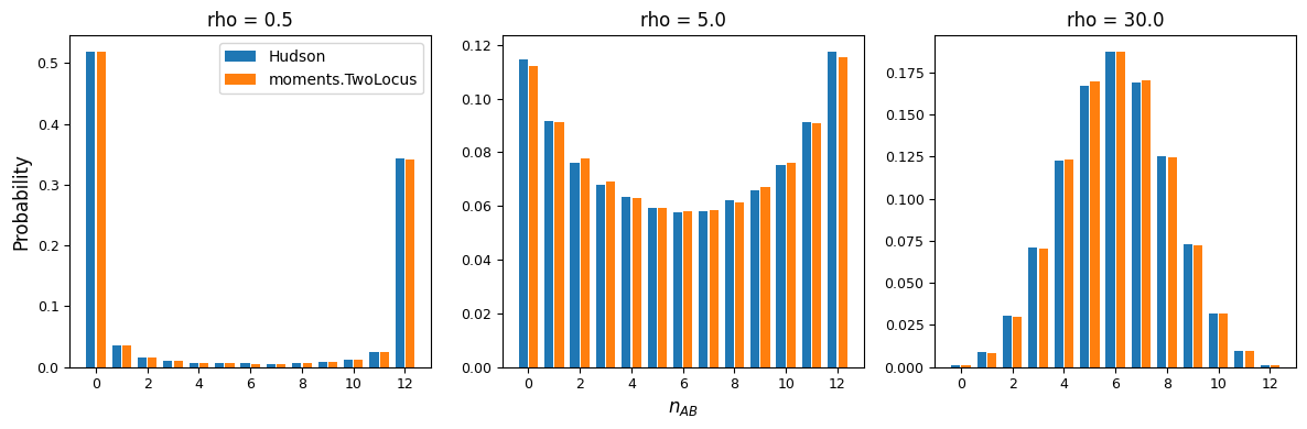
For low recombination rates, the marginal distribution of AB haplotypes is skewed
toward the maximum or minimum number of copies, resulting in higher LD, while for larger
recombination rates, the distribution of \(n_{AB}\) is concentrated around frequencies
that result in low levels of LD. We can also see that moments.TwoLocus agrees well
with Hudson’s results under neutrality and steady state demography.
Note
Below, we’ll be revisiting these same statistics and seeing how various models of selection at the two loci, as well as non-steady state demography, distort the expected distributions.
How does selection interact across multiple loci?
There has been a recent resurgence of interest in learning about the interaction of
selection at two or more loci (e.g., for studies within the past few years, see
[Sohail], [Garcia], [Sandler], [Good]). This has largely been driven by the
relatively recent availability of large-scale sequencing datasets that allow us to
observe patterns of allele frequencies and LD for negatively selected loci that may
be segregating at very low frequencies in a population. Some of these studies are
theory-driven (e.g., [Good]), while others rely on forward Wright-Fisher simulators
(such as SLiM or fwdpy11) to compare observed patterns between data and
simulation.
These approaches have their limitations: analytical results are largely constrained to simple selection scenarios and steady-state demography, while simulation studies are computationally expensive and thus often end up limited to still a handful of selection and demographic scenarios. Numerical approaches to compute expectations of statistics of interest could therefore provide a far more efficient way to compute explore parameter regimes and compare model expectations to data in inference frameworks.
Here, we’ll explore a few selection models, including both dominance and epistatic effects, that theory predicts should result in different patterns of LD between two selected loci. We first describe the selection models, and then we compare their expected patterns of LD.
Selection models at two loci
At a single locus, the effects of selection and dominance are captured by the selection coefficient \(s\) and the dominance coefficient \(h\), so that fitnesses of the diploid genotypes are given by
Genotype |
Relative fitness |
aa |
\(1\) |
Aa |
\(1 + 2hs\) |
AA |
\(1 + 2s\) |
If \(h = 1/2\), i.e. selection is additive, this model reduces to a haploid selection model where genotype A has relative fitness \(1 + s\) compared to a.
Additive selection, no epistasis
Additive selection models for two loci, like in the single-locus case, reduce to haploid-based models, where we only need to know the relative fitnesses of the two-locus haplotypes AB, Ab, aB, and ab. When we say “no epistasis,” we typically mean that the relative fitness of an individual carrying both derived alleles (AB) is additive across loci, so that if \(s_A\) is the selection coefficient at the left (A/a) locus, and \(s_B\) is the selection coefficient at the right (B/b) locus, then \(s_{AB} = s_A + s_B\).
Genotype |
Relative fitness |
ab |
\(1\) |
Ab |
\(1 + s_A\) |
aB |
\(1 + s_B\) |
AB |
\(1 + s_{AB} = 1 + s_A + s_B\) |
Additive selection with epistasis
Epistasis is typically modeled as a factor \(\epsilon\) that either increases or decreases the selection coefficient for the AB haplotype, so that \(s_{AB} = s_A + s_B + \epsilon\). If \(|s_{AB}| > |s_A| + |s_A|\), i.e. the fitness effect of the AB haplotype is greater than the sum of the effect of the Ab and aB haplotypes, the effect is called synergistic epistasis, and if \(|s_{AB}| < |s_A| + |s_A|\), it is refered to as antagonistic epistasis.
Genotype |
Relative fitness |
ab |
\(1\) |
Ab |
\(1 + s_A\) |
aB |
\(1 + s_B\) |
AB |
\(1 + s_{AB} = 1 + s_A + s_B + \epsilon\) |
Simple dominance, no epistasis
Epistasis is the non-additive interaction of selective effects across loci. The non-additive effect of selection within a locus is called dominance, when \(s_{AA} \not= 2s_{Aa}\). Without epistasis, so that \(s_{AB}=s_{A}+s_{B}\), and allowing for different selection and dominance coefficients at the two loci, the fitness effects for two-locus diploid genotypes takes a simple form analogous to the single-locus case with dominance. Here, we define the relative fitnesses of two-locus diploid genotypes, which relies on the selection and dominance coefficients at the left and right loci:
Genotype |
Relative fitness |
aabb |
\(1\) |
Aabb |
\(1 + 2 h_A s_A\) |
AAbb |
\(1 + 2 s_A\) |
aaBb |
\(1 + 2 h_B s_B\) |
AaBb |
\(1 + 2 h_A s_A + 2 h_B s_B\) |
AABb |
\(1 + 2 s_A + 2 h_B s_B\) |
aaBB |
\(1 + 2 s_B\) |
AaBB |
\(1 + 2 h_A s_A + 2 s_B\) |
AABB |
\(1 + 2 s_A + 2 s_B\) |
Both dominance and epistasis
As additional non-additive interactions are introduced, it gets more difficult to succinctly define general selection models with few parameters. A general selection model that is flexible could simply define a selection coefficient for each two-locus diploid genotype, in relation to the double wild-type homozygote (aabb). That is, define \(s_{Aabb}\) as the selection coefficient for the Aabb genotype, \(s_{AaBb}\) the selection coefficient for the AaBb genotype, and so on.
Gene-based dominance
In the above model, fitness is determined by combined hetero-/homozygosity at the two loci, but it does not make a distinction between the different ways that double heterozygotes (AaBb) could arise. Instead, we could imagine a model where diploid individual fitnesses depend on the underlying haplotypes, i.e. whether selected mutations at the two loci are coupled on the same background or are on different haplotypes.
For example, consider loss-of-function mutations in coding regions. Such mutations tend to be severely damaging. We could think of the situation where diploid individual fitness is strongly reduced when both copies carry a loss-of-function mutation, but much less reduced if the individual has at least one copy without a mutation. In this scenario, the haplotype combination Ab / aB will confer more reduced fitness compared to the combination AB / ab, even though both are double heterozygote genotypes.
Perhaps the simplest model for gene-based dominance assumes that derived mutations at the two loci (A and B) carry the same fitness cost, and fitness depends on the number of haplotype copies within a diploid individual that have at least one such mutation. This model requires just two parameters, a single selection coefficient s and a single dominance coefficient h:
Genotype |
Relative fitness |
ab / ab |
\(1\) |
Ab / ab |
\(1 + 2 h s\) |
aB / ab |
\(1 + 2 h s\) |
AB / ab |
\(1 + 2 h s\) |
Ab / Ab |
\(1 + 2 s\) |
aB / aB |
\(1 + 2 s\) |
Ab / aB |
\(1 + 2 s\) |
AB / Ab |
\(1 + 2 s\) |
AB / aB |
\(1 + 2 s\) |
AB / AB |
\(1 + 2 s\) |
Note
Cite [Sanjak]
How do different selection models affect expected LD statistics?
Here, we will examine some relatively simple models in order to gain some intuition about how selection, along with recombination and size changes, affect expected patterns of LD, such as the decay curve of \(\sigma_d^2\) and Hudson-style slices in the two-locus sampling distribution. The selection coefficients will be equal at the two loci, so that the only selection parameters that change will be the selection models (dominance and epistasis).
Additive selection with and without epistasis
Let’s first see how simple, additive selection distorts expected LD away from neutral expectations at steady state. Plotted below are decay curves for both \(\sigma_d^2\) and \(\sigma_d^2 = {\mathbb{E}[D]}{\mathbb{E}[p(1-p)q(1-q)]}\), a common signed LD statistic.
For each parameter pair of selection coefficient \(\gamma = 2 N_e s\) and \(rho\), we use the “helper” function that creates the input selection parameters for the AB, Ab, and aB haplotypes, and then simulate the equilibrium two-locus sampling distribution:
sel_params = moments.TwoLocus.Util.additive_epistasis(gamma, epsilon=0)
# epsilon=0 means no epistasis, so s_AB = s_A + s_B
F = moments.TwoLocus.Demographics.equilibrium(n, rho=rho, sel_params=sel_params)
sigma_d1 = F.D() / F.pi2()
sigma_d2 = F.D2() / F.pi2()
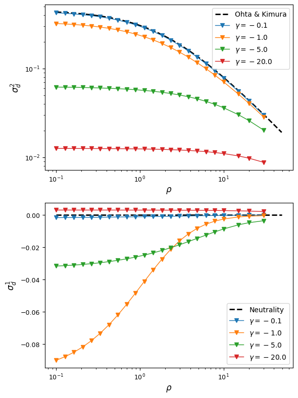
Already with this very simple selection model (no epistasis, no dominance, equal selection at both loci), we find some interesting behavior. For very strong or very week selection, signed-LD remains close to zero, but for intermediate selection, average \(D\) can be significantly negative. As fitness effects get stronger, \(\sigma_d^2\) is reduced dramatically compare to neutral expectations.
Todo
Plots of frequency conditioned LD.
The “helper” function that we used above converts input \(\gamma\) and \(\epsilon\)
to the selection parameters that are passed to moments.TwoLocus.Demographics functions.
The additive epistasis model implemented in the helper function
(moments.TwoLocus.Util.additive_epistasis) returns
\([(1+\epsilon)(\gamma_A + \gamma_B), \gamma_A, \gamma_B]\), so that if
\(\epsilon > 0\), we have synergistic epistasis, and if \(\epsilon < 0\), we
have antagonistic epistasis. Any value of \(\epsilon\) is permitted, and note that if
\(\epsilon\) is less than \(-1\), we get reverse-sign epistasis.
We’ll focus on two selection regions: mutations that are slightly deleterious with \(\gamma=1\), and stronger selection with \(\gamma=20\). With an effective population size of 10,000, note that \(\gamma=20\) corresponds to \(s=0.001\) - by no means a lethal mutation, but strong enough to see some interesting differences between selection regimes.
Below we again plot \(\sigma_d^2\) and \(\sigma_d^1\) for each set of parameters:
gammas = [-1, -20]
epsilons = [-1, -0.5, 0, 0.5, 1]
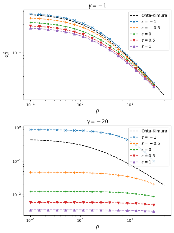
From this, we can see that synergistic epistasis decreases \(\sigma_d^2\) and antagonistic epistasis increases it above expectations for \(\epsilon=0\). For signed LD, however, both positive and negative \(\epsilon\) push \(\sigma_d^1\) farther away from zero:

As expected, negative \(\epsilon\) (i.e. selection against the AB haplotype is less strong than the sum of selection against A and B) leads to an excess of coupling LD (pairs with more AB and ab haplotypes) than repulsion LD (pairs with more Ab and aB haplotypes).
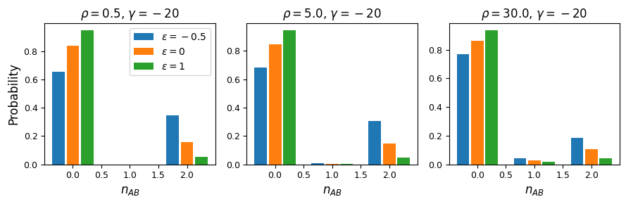
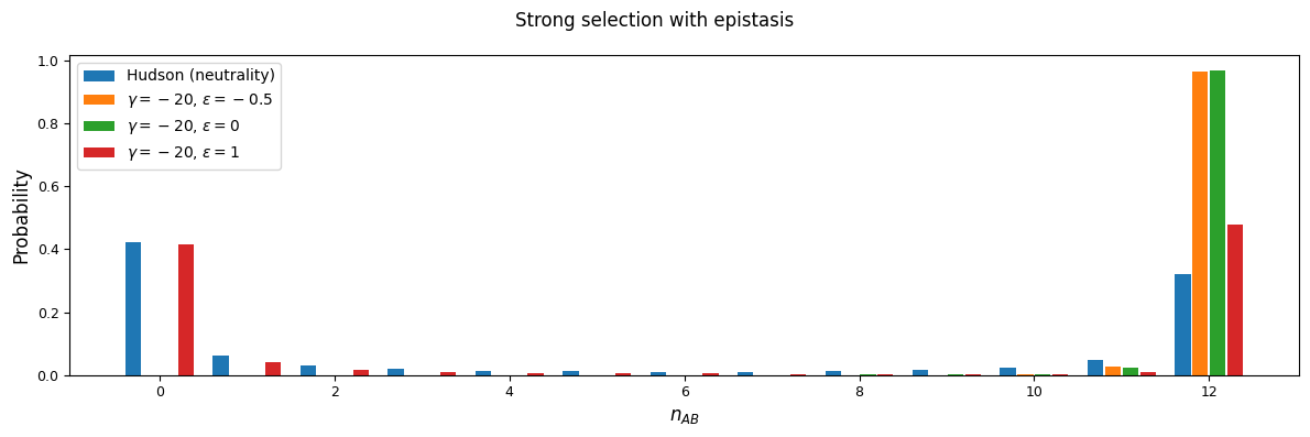
We can see this effect more clearly by looking at a slice in the two-locus sampling distribution. Since we’re considering negative selection, we’ll look at entries in the sampling distribution with low frequencies at the two loci. For doubletons at both sites:
rhos = [0.5, 5.0, 30.0]
n = 30
nA = 2
nB = 2

epsilon = [-0.5, 0, 1]

fig = plt.figure(figsize=(9, 3))
for ii, rho in enumerate(rhos):
    pABs = {}
    for eps in epsilon:
        sel_params = moments.TwoLocus.Util.additive_epistasis(gammas[0], epsilon=eps)
        # F = moments.TwoLocus.Demographics.equilibrium(
        #     n, rho=rho, sel_params=sel_params)
        F = pickle.load(gzip.open(
            f"./data/two-locus/eq.n_{n}.rho_{rho}.sel_"
            + "_".join([str(s) for s in sel_params])
            + ".fs.gz",
            "rb"))
        counts, pAB = moments.TwoLocus.Util.pAB(F, nA, nB)
        pABs[eps] = pAB / pAB.sum()
    ax = plt.subplot(1, 3, ii + 1)
    ax.bar(counts - 0.25, pABs[epsilon[0]], width=0.22, label=rf"$\epsilon={epsilon[0]}$")
    ax.bar(counts, pABs[epsilon[1]], width=0.22, label=rf"$\epsilon={epsilon[1]}$")
    ax.bar(counts + 0.25, pABs[epsilon[2]], width=0.22, label=rf"$\epsilon={epsilon[2]}$")

    ax.set_title(rf"$\rho = {rho}$, $\gamma = {gammas[0]}$")
    ax.set_xlabel(r"$n_{AB}$")
    if ii == 0:
        ax.legend()
        ax.set_ylabel("Probability")
fig.tight_layout()
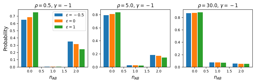
fig = plt.figure(figsize=(9, 3))
for ii, rho in enumerate(rhos):
    pABs = {}
    for eps in epsilon:
        sel_params = moments.TwoLocus.Util.additive_epistasis(gammas[1], epsilon=eps)
        # F = moments.TwoLocus.Demographics.equilibrium(
        #     n, rho=rho, sel_params=sel_params)
        F = pickle.load(gzip.open(
            f"./data/two-locus/eq.n_{n}.rho_{rho}.sel_"
            + "_".join([str(s) for s in sel_params])
            + ".fs.gz",
            "rb"))
        counts, pAB = moments.TwoLocus.Util.pAB(F, nA, nB)
        pABs[eps] = pAB / pAB.sum()
    ax = plt.subplot(1, 3, ii + 1)
    ax.bar(counts - 0.25, pABs[epsilon[0]], width=0.22, label=rf"$\epsilon={epsilon[0]}$")
    ax.bar(counts, pABs[epsilon[1]], width=0.22, label=rf"$\epsilon={epsilon[1]}$")
    ax.bar(counts + 0.25, pABs[epsilon[2]], width=0.22, label=rf"$\epsilon={epsilon[2]}$")

    ax.set_title(rf"$\rho = {rho}$, $\gamma = {gammas[1]}$")
    ax.set_xlabel(r"$n_{AB}$")
    if ii == 0:
        ax.legend()
        ax.set_ylabel("Probability")
fig.tight_layout()
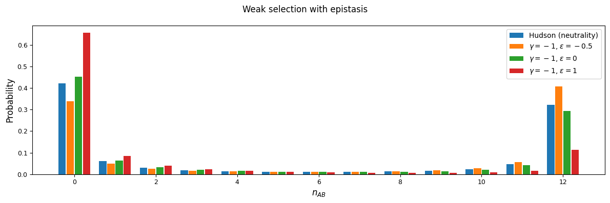
And while very few mutations will reach high frequency, we can also look at the case with \(n_A=15\) and \(n_B=12\) in a sample size of 30. Here, because selection and recombination require the jackknife approximation which works better with larger sample sizes, we solved for the equilibrium distribution using size \(n=60\) and then projected to size 30.
n = 60
n_proj = 30
nA = 15
nB = 12
rho = 1

F = moments.TwoLocus.Demographics.equilibrium(n, rho=rho, sel_params=sel_params)
# by default, we usually cache projection steps, but set cache=False here to
# save on memory usage
F_proj = F.project(n_proj, cache=False)
counts, pAB = moments.TwoLocus.Util.pAB(F_proj, nA, nB)
pAB /= pAB.sum()
Dominance
We again assume fitness effects are the same at both loci, and now explore how dominance
affects LD. We’ll start by looking at the “simple” dominance model without epistasis, so
that fitness effects are additive across loci. When simulating with dominance, the selection
model no longer collapses to a haploid model, but instead we need to specify the selection
coefficients for each possible diploid haplotype pair AB/AB, AB/Ab, etc. We’ll use
another helper function to generate those selection coefficients and pass them to the
sel_params_general keyword argument.
For example, to simulate the equilibrium distribution with selection coefficient -5 and dominance coefficient 0.1 under the simple dominance model:
gamma = -5
h = 0.1
sel_params = moments.TwoLocus.Util.simple_dominance(gamma, h=h)
F = moments.TwoLocus.Demographics.equilibrium(n, rho, sel_params_general=sel_params)
Let’s look at how \(\sigma_d^2\) and \(\sigma_d^1\) are affected by dominance.
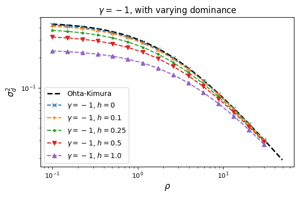
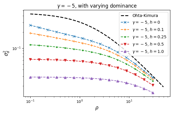
Squared LD (\(\sigma_d^2\)) is increased for recessive variants, while pairs of dominant mutations reduce it below expectations for additive variants.
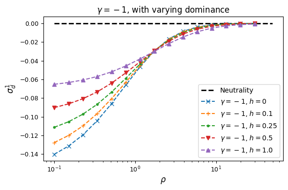
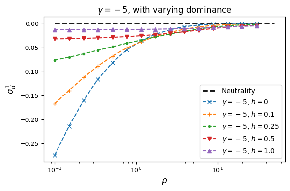
Similarly, recessive mutations lead to larger average negative signed LD. However, this pattern also depends on the underlying selection coefficient, with LD decay curves that can vary qualitatively for different selection coefficients and recombination rates between loci, even when dominance is equivalent.
Todo
Relate to associative overdominance work, e.g. Charlesworth, and Hill-Robertson interference.
Gene-based dominance
Todo
All the comparisons, show LD curves and expectations for signed LD, depending on the selection model, maybe explore how population size changes distort these expectations.
Non-steady-state demography
\(\mathcal{K}\)
Todo
Are any of these statistics quite sensitive to bottlenecks or expansions?
Todo
Discussion on what we can expect to learn from signed LD-based inferences. Are the various selection models and demography hopelessly confounded?
References
Garcia, Jesse A., and Kirk E. Lohmueller. “Negative linkage disequilibrium between amino acid changing variants reveals interference among deleterious mutations in the human genome.” bioRxiv (2020).
Hudson, Richard R. “Two-locus sampling distributions and their application.” Genetics 159.4 (2001): 1805-1817.
Ohta, Tomoko, and Motoo Kimura. “Linkage disequilibrium between two segregating nucleotide sites under the steady flux of mutations in a finite population.” Genetics 68.4 (1971): 571.
Ragsdale, Aaron P. and Ryan N. Gutenkunst. “Inferring demographic history using two-locus statistics.” Genetics 206.2 (2017): 1037-1048.
Ragsdale, Aaron P. and Simon Gravel. “Models of archaic admixture and recent history from two-locus statistics.” PLoS Genetics 15.8 (2019): e1008204.
Sandler, George, Stephen I. Wright, and Aneil F. Agrawal. “Using patterns of signed linkage disequilibria to test for epistasis in flies and plants.” bioRxiv (2020).
Sanjak, Jaleal S., Anthony D. Long, and Kevin R. Thornton. “A model of compound heterozygous, loss-of-function alleles is broadly consistent with observations from complex-disease GWAS datasets.” PLoS genetics 13.1 (2017): e1006573.
Sohail, Mashaal, et al. “Negative selection in humans and fruit flies involves synergistic epistasis.” Science 356.6337 (2017): 539-542.